Using JupyterLab

Overview

Teaching: 10 min
Exercises: 0 min

Questions

• How can I use JupyterLab for Climate Data Analysis

Objectives

• Learn key features of JupyterLab to use for Climate Data Analysis

JupyterLab (Jupyter Notebook)

JupyterLab allows us to create Jupyter Notebooks which can contain a combination of code, figures, links, formatted text, and even LaTex equations.

It is also a web-based programming interface for mutiple languages (e.g. Python, R, Julia…). We will use it as our Python programming interface.

Because it also allows figures, links, text, and equations in addition to code, it is very useful for use in research allowing all your information related to your research to be kept together rather than in separate documents. It’s like a fancy, high-tech research journal!

Creating and working with a Jupyter Notebook

First, let’s create a new Jupyter Notebook by clicking in the menu bar File->New->Notebook or in the Launcher clicking on Python 3 (ORC) in the row labeled Notebook This creates a new notebook with a default title Untitled.ipynb or Untitled#.ipynb. Note that Jupyter Notebooks end in .ipynb

Change the name of your notebook to PracticeNotebook.ipynb by clicking File->Save Notebook As

Each rectangular box in your notebook is called a cell it contains a block of code, Markdown text, or Raw text. What a cell contains is indicated in the menu above.

To determine what kind of code our notebook will contain and run, the kernel is shown in the upper right. This notebook contains Python 3 code. (ORC) is the environment, which has a preset list of libraries available to import. Later we will learn how to make and modify environments.

What is Markdown?

Markdown is a formatting language that allows you to provide basic formatted text (e.g. bold, italics, links, different sized font, and LaTeX equations). It’s not as fancy as what you could do with a word processor, but for documenting projects in Jupyter notebooks, it gets the job done nicely!

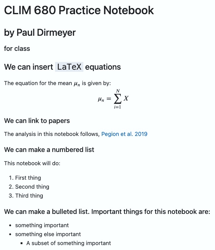
As an example, let’s type the following in a cell and change the cell to Markdown:

# CLIM 680 Practice Notebook
## by {your name here}
#### for class

### We can insert `LaTeX` equations
The equation for the mean $\mu_n$ is given by: 
$$ \mu_n=\sum_{i=1}^{N}X $$

#### We can link to papers
The analysis in this notebook follows, [Pegion et al. 2019](https://doi.org/10.1175/BAMS-D-18-0270.1)

#### We can make a numbered list 
This notebook will do:
1. First thing
2. Second thing
3. Third thing

#### We can make a bulleted list. Important things for this notebook are:
* something important
* something else important
  * A subset of something important

Once you are finished, run the cell by either:

• Clicking the “play” button ▶ at top of the tab

• Typing shift-return

Your result should look something like this once you run the cell:

What is LaTeX (and why do you type it like that)?

LaTeX (pronounced “lah-tek” or “lay-tek” but never “lay-teks”) is a simple text-based protocol for encoding text to be formatted for publication printing. It evolved from the days before word processors, and even before GUI operating systems like Windows and Mac OS, when everything about computing had to be typed at the command like of a terminal window.

LaTeX was started in the mid 1980s as a publication-quality protocol for encoding typesetting commands as a set of special codes embedded within normal text. It is still very popular to this day, especially with mathematicians, physicists and others who write a lot of equations. It’s system is considered easier and faster to type than the equation coding systems of apps like Microsoft Word. In fact, it’s so popular that modern versions of Word allow users the option to use LaTeX syntax in its own equation editor.

Here is a handy guide for rendering mathematical symbols and expressions in LaTeX, which will also render nicely in markdown cells within Jupyter notebooks.

Key Points

• JupyterLab can be used as a Python programming environment

• You can create notebooks with codes, figures, links, text, and equations

• You can run your codes in JupyterLab cell by cell

Repeating Actions with Loops

Overview

Teaching: 25 min
Exercises: 5 min

Questions

• How can I do the same operations on many different values?

Objectives

• Explain what a for loop does.

• Correctly write for loops to repeat simple calculations.

• Trace changes to a loop variable as the loop runs.

• Trace changes to other variables as they are updated by a for loop.

In the last episode, we wrote Python code that plots values of interest from our first inflammation dataset (inflammation-01.csv), which revealed some suspicious features in it.

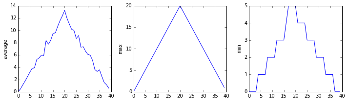
We have a dozen data sets right now, though, and more on the way. We want to create plots for all of our data sets with a single statement. To do that, we’ll have to teach the computer how to repeat things.

An example task that we might want to repeat is printing each character in a word on a line of its own.

word = 'lead'

In Python, a string is basically an ordered collection of characters, and every character has a unique number associated with it – its index. This means that we can access characters in a string using their indices. For example, we can get the first character of the word 'lead', by using word[0]. One way to print each character is to use four print statements:

print(word[0])
print(word[1])
print(word[2])
print(word[3])

l
e
a
d

This is a bad approach for three reasons:

1. Not scalable. Imagine you need to print characters of a string that is hundreds of letters long. It might be easier to type them in manually.

2. Difficult to maintain. If we want to decorate each printed character with an asterisk or any other character, we would have to change four lines of code. While this might not be a problem for short strings, it would definitely be a problem for longer ones.

3. Fragile. If we use it with a word that has more characters than what we initially envisioned, it will only display part of the word’s characters. A shorter string, on the other hand, will cause an error because it will be trying to display part of the string that doesn’t exist.

word = 'tin'
print(word[0])
print(word[1])
print(word[2])
print(word[3])

t
i
n

---------------------------------------------------------------------------
IndexError                                Traceback (most recent call last)
<ipython-input-3-7974b6cdaf14> in <module>()
      3 print(word[1])
      4 print(word[2])
----> 5 print(word[3])

IndexError: string index out of range

Here’s a better approach:

word = 'lead'
for char in word:
    print(char)

l
e
a
d

This is shorter — certainly shorter than something that prints every character in a hundred-letter string — and more robust as well:

word = 'oxygen'
for char in word:
    print(char)

o
x
y
g
e
n

The improved version uses a for loop to repeat an operation — in this case, printing — once for each thing in a sequence. The general form of a loop is:

for variable in collection:
    # do things using variable, such as print

Using the oxygen example above, the loop might look like this:

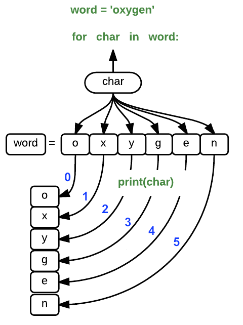
where each character (char) in the variable word is looped through and printed one character after another. The numbers in the diagram denote which character was printed (0 being the first loop cycle, and 5 in the final or sixth loop).

We can call the loop variable anything we like, but there must be a colon at the end of the line starting the loop, and we must indent anything we want to run inside the loop. Unlike many other languages, there is no command to signify the end of the loop body (e.g. end for); what is indented after the for statement belongs to the loop.

What’s in a name?

In the example above, the loop variable was given the name char as a mnemonic; it is short for ‘character’. We can choose any name we want for variables. We can even call our loop variable banana, as long as we use this name consistently:

word = 'oxygen'
for banana in word:
    print(banana)

o
x
y
g
e
n

It is a good idea to choose variable names that are meaningful, otherwise it would be more difficult to understand what the loop is doing.

Here’s another loop that repeatedly updates a variable:

length = 0
for vowel in 'aeiou':
    length = length + 1
print('There are', length, 'vowels')

There are 5 vowels

It’s worth tracing the execution of this little program step by step. Since there are five characters in 'aeiou', the statement on line 3 will be executed five times. The first time around, length is zero (the value assigned to it on line 1) and vowel is 'a'. The statement adds 1 to the old value of length, producing 1, and updates length to refer to that new value. The next time around, vowel is 'e' and length is 1, so length is updated to be 2. After three more updates, length is 5; since there is nothing left in 'aeiou' for Python to process, the loop finishes and the print statement on line 4 tells us our final answer.

Note that a loop variable is a variable that’s being used to record progress in a loop. It still exists after the loop is over, and we can re-use variables previously defined as loop variables as well:

letter = 'z'
for letter in 'abc':
    print(letter)
print('after the loop, letter is', letter)

a
b
c
after the loop, letter is c

Note also that finding the length of a string is such a common operation that Python actually has a built-in function to do it called len:

print(len('aeiou'))

5

len is much faster than any function we could write ourselves, and much easier to read than a two-line loop; it will also give us the length of many other things that we haven’t met yet, so we should always use it when we can.

From 1 to N

Python has a built-in function called range that generates a sequence of numbers. range can accept 1, 2, or 3 parameters.

• If one parameter is given, range generates a sequence of that length, starting at zero and incrementing by 1. For example, range(3) produces the numbers 0, 1, 2.
• If two parameters are given, range starts at the first and ends just before the second, incrementing by one. For example, range(2, 5) produces 2, 3, 4.
• If range is given 3 parameters, it starts at the first one, ends just before the second one, and increments by the third one. For example, range(3, 10, 2) produces 3, 5, 7, 9.

Using range, write a loop that uses range to print the first 3 natural numbers:

1
2
3

Solution

for number in range(1, 4):
    print(number)

Understanding the loops

Given the following loop:

word = 'oxygen'
for char in word:
    print(char)

How many times is the body of the loop executed?

• 3 times
• 4 times
• 5 times
• 6 times

Solution

The body of the loop is executed 6 times.

Computing Powers With Loops

Exponentiation is built into Python:

print(5 ** 3)

125

Write a loop that calculates the same result as 5 ** 3 using multiplication (and without exponentiation).

Solution

result = 1
for number in range(0, 3):
    result = result * 5
print(result)

Reverse a String

Knowing that two strings can be concatenated using the + operator, write a loop that takes a string and produces a new string with the characters in reverse order, so 'Newton' becomes 'notweN'.

Solution

newstring = ''
oldstring = 'Newton'
for char in oldstring:
    newstring = char + newstring
print(newstring)

Computing the Value of a Polynomial

The built-in function enumerate takes a sequence (e.g. a list) and generates a new sequence of the same length. Each element of the new sequence is a pair composed of the index (0, 1, 2,…) and the value from the original sequence:

for idx, val in enumerate(a_list):
    # Do something using idx and val

The code above loops through a_list, assigning the index to idx and the value to val.

Suppose you have encoded a polynomial as a list of coefficients in the following way: the first element is the constant term, the second element is the coefficient of the linear term, the third is the coefficient of the quadratic term, etc.

x = 5
coefs = [2, 4, 3]
y = coefs[0] * x**0 + coefs[1] * x**1 + coefs[2] * x**2
print(y)

97

Write a loop using enumerate(coefs) which computes the value y of any polynomial, given x and coefs.

Solution

y = 0
for idx, coef in enumerate(coefs):
    y = y + coef * x**idx

Key Points

• Use for variable in sequence to process the elements of a sequence one at a time.

• The body of a for loop must be indented.

• Use len(thing) to determine the length of something that contains other values.

Storing Multiple Values in Lists

Overview

Teaching: 25 min
Exercises: 10 min

Questions

• How can I store many values together?

Objectives

• Explain what a list is.

• Create and index lists of simple values.

• Change the values of individual elements

• Append values to an existing list

• Reorder and slice list elements

• Create and manipulate nested lists

Similar to a string that can contain many characters, a list is a container that can store many values, called items. Unlike NumPy arrays, lists are built into the language (so we don’t have to load a library to use them). We create a list by putting values inside square brackets and separating the values with commas:

odds = [1, 3, 5, 7]
print('odds are:', odds)

odds are: [1, 3, 5, 7]

We can access items of a list using indices – numbered positions of items in the list. These positions are numbered starting at 0, so the first item has an index of 0.

print('first item:', odds[0])
print('last item:', odds[3])
print('"-1" item:', odds[-1])

first item: 1
last item: 7
"-1" item: 7

Yes, we can use negative numbers as indices in Python. When we do so, the index -1 gives us the last item in the list, -2 the second to last, and so on. Because of this, odds[3] and odds[-1] point to the same item here.

If we loop over a list, the loop variable is assigned to its items one at a time:

for number in odds:
    print(number)

1
3
5
7

There is one important difference between lists and strings: we can change the items in a list, but we cannot change individual characters in a string. For example:

names = ['Curie', 'Darwing', 'Turing']  # typo in Darwin's name
print('names is originally:', names)
names[1] = 'Darwin'  # correct the name
print('final value of names:', names)

names is originally: ['Curie', 'Darwing', 'Turing']
final value of names: ['Curie', 'Darwin', 'Turing']

works, but:

name = 'Darwin'
name[0] = 'd'

---------------------------------------------------------------------------
TypeError                                 Traceback (most recent call last)
<ipython-input-8-220df48aeb2e> in <module>()
      1 name = 'Darwin'
----> 2 name[0] = 'd'

TypeError: 'str' object does not support item assignment

does not.

Ch-Ch-Ch-Ch-Changes

Data which can be modified in place is called mutable, while data which cannot be modified is called immutable. Strings and numbers are immutable. This does not mean that variables with string or number values are constants, but when we want to change the value of a string or number variable, we can only replace the old value with a completely new value.

Lists and arrays, on the other hand, are mutable: we can modify them after they have been created. We can change individual items, append new items, or reorder the whole list. For some operations, like sorting, we can choose whether to use a function that modifies the data in-place or a function that returns a modified copy and leaves the original unchanged.

Be careful when modifying data in-place. If two variables refer to the same list, and you modify the list contents, it will change for both variables!

salsa = ['peppers', 'onions', 'cilantro', 'tomatoes']
my_salsa = salsa        # <-- my_salsa and salsa point to the *same* list data in memory
salsa[0] = 'hot peppers'
print('Ingredients in my salsa:', my_salsa)

Ingredients in my salsa: ['hot peppers', 'onions', 'cilantro', 'tomatoes']

If you want variables with mutable values to be independent, you must make a copy of the list when you assign it. As this is Python, there are multiple ways to do this. For instance:

salsa = ['peppers', 'onions', 'cilantro', 'tomatoes']
my_salsa = list(salsa)        # <-- makes a *copy* of the list
salsa[0] = 'hot peppers'
print('Ingredients in my salsa:', my_salsa)

Ingredients in my salsa: ['peppers', 'onions', 'cilantro', 'tomatoes']

Alternatively, many objects including lists have a copy method:

salsa = ['peppers', 'onions', 'cilantro', 'tomatoes']
my_salsa = salsa.copy()        # <-- also makes a *copy* of the list
salsa[0] = 'hot peppers'
print('Ingredients in my salsa:', my_salsa)

Ingredients in my salsa: ['peppers', 'onions', 'cilantro', 'tomatoes']

Because of pitfalls like this, code which modifies data in place can be more difficult to understand. However, it is often far more efficient to modify a large data structure in place than to create a modified copy for every small change. You should consider both of these aspects when writing your code.

Nested Lists

Since a list can contain any Python variables, it can even contain other lists.

For example, we could represent the products in the shelves of a small grocery shop:

x = [['pepper', 'zucchini', 'onion'],
     ['cabbage', 'lettuce', 'garlic'],
     ['apple', 'pear', 'banana']]

Here is a visual example of how indexing a list of lists x works:

Using the previously declared list x, these would be the results of the index operations shown in the image:

print([x[0]])

[['pepper', 'zucchini', 'onion']]

print(x[0])

['pepper', 'zucchini', 'onion']

print(x[0][0])

'pepper'

You may recogize that a list is like a series in mathematics, and a list of lists is like a 2-D array. The analogy continues - a list of lists of lists is like a 3-D array, etc.

Thanks to Hadley Wickham for the image above.

Heterogeneous Lists

Lists in Python can contain items of different types. Example:

sample_ages = [10, 12.5, 'Unknown']

There are many ways to change the contents of lists besides assigning new values to individual items:

odds.append(11)
print('odds after adding a value:', odds)

odds after adding a value: [1, 3, 5, 7, 11]

removed_element = odds.pop(0)
print('odds after removing the first element:', odds)
print('removed_element:', removed_element)

odds after removing the first element: [3, 5, 7, 11]
removed_element: 1

odds.reverse()
print('odds after reversing:', odds)

odds after reversing: [11, 7, 5, 3]

While modifying in place, it is useful to remember that Python treats lists in a slightly counter-intuitive way.

As we saw earlier, when we modified the salsa list item in-place, if we make a list, (attempt to) copy it and then modify this list, we can cause all sorts of trouble. This also applies to modifying the list using the above functions:

odds = [1, 3, 5, 7]
primes = odds
primes.append(2)
print('primes:', primes)
print('odds:', odds)

primes: [1, 3, 5, 7, 2]
odds: [1, 3, 5, 7, 2]

This is because Python stores a list in memory, and then can use multiple names to refer to the same list, the same location in memory. If all we want to do is copy a (simple) list, we can again use the list function (or more generally, the copy() method), so we do not modify a list we did not mean to:

odds = [1, 3, 5, 7]
primes = list(odds)
primes.append(2)
print('primes:', primes)
print('odds:', odds)

primes: [1, 3, 5, 7, 2]
odds: [1, 3, 5, 7]

Turn a String Into a List

Use a for-loop to convert the string “hello” into a list of letters:

['h', 'e', 'l', 'l', 'o']

Hint: You can create an empty list like this:

my_list = []

Solution

my_list = []
for char in 'hello':
    my_list.append(char)
print(my_list)

Subsets of lists and strings can be accessed by specifying ranges of values in brackets, similar to how we accessed ranges of positions in a NumPy array. This is commonly referred to as “slicing” the list/string.

binomial_name = 'Drosophila melanogaster'
group = binomial_name[0:10]
print('group:', group)

species = binomial_name[11:23]
print('species:', species)

chromosomes = ['X', 'Y', '2', '3', '4']
autosomes = chromosomes[2:5]
print('autosomes:', autosomes)

last = chromosomes[-1]
print('last:', last)

group: Drosophila
species: melanogaster
autosomes: ['2', '3', '4']
last: 4

Slicing From the End

Use slicing to access only the last four characters of a string or entries of a list.

string_for_slicing = 'Observation date: 02-Feb-2013'
list_for_slicing = [['fluorine', 'F'],
                    ['chlorine', 'Cl'],
                    ['bromine', 'Br'],
                    ['iodine', 'I'],
                    ['astatine', 'At']]

'2013'
[['chlorine', 'Cl'], ['bromine', 'Br'], ['iodine', 'I'], ['astatine', 'At']]

Would your solution work regardless of whether you knew beforehand the length of the string or list (e.g. if you wanted to apply the solution to a set of lists of different lengths)? If not, try to change your approach to make it more robust.

Hint: Remember that indices can be negative as well as positive

Solution

Use negative indices to count elements from the end of a container (such as items in a list or characters in a string):

string_for_slicing[-4:]
list_for_slicing[-4:]

Non-Continuous Slices

So far we’ve seen how to use slicing to take single blocks of successive entries from a sequence. But what if we want to take a subset of entries that aren’t next to each other in the sequence?

If the elements to be chosen are evenly spaced, you can achieve this by providing a third argument to the range within the brackets, called the step size. The example below shows how you can take every third entry in a list:

primes = [2, 3, 5, 7, 11, 13, 17, 19, 23, 29, 31, 37]
subset = primes[0:12:3]
print('subset', subset)

subset [2, 7, 17, 29]

Notice that the slice taken begins with the first entry in the range, followed by entries taken at equally-spaced intervals (the steps) thereafter. If you wanted to begin the subset with the third entry, you would need to specify that as the starting point of the sliced range:

primes = [2, 3, 5, 7, 11, 13, 17, 19, 23, 29, 31, 37]
subset = primes[2:12:3]
print('subset', subset)

subset [5, 13, 23, 37]

Use the step size argument to create a new string that contains only every other character in the string “In an octopus’s garden in the shade”. Start with creating a variable to hold the string:

beatles = "In an octopus's garden in the shade"

What slice of beatles will produce the following output (i.e., the first character, third character, and every other character through the end of the string)? ~~~ I notpssgre ntesae ~~~

Solution

To obtain every other character you need to provide a slice with the step size of 2:

beatles[0:35:2]

You can also leave out the beginning and end of the slice to take the whole string and provide only the step argument to go every second element:

beatles[::2]

If you want to take a slice from the beginning of a sequence, you can safely omit the first index in the range:

date = 'Monday 4 January 2016'
day = date[0:6]
print('Using 0 to begin range:', day)
day = date[:6]
print('Omitting beginning index:', day)

Using 0 to begin range: Monday
Omitting beginning index: Monday

And similarly, you can safely omit the ending index in the range to take a slice to the very end of the sequence:

months = ['jan', 'feb', 'mar', 'apr', 'may', 'jun', 'jul', 'aug', 'sep', 'oct', 'nov', 'dec']
sond = months[8:12]
print('With known last position:', sond)
sond = months[8:len(months)]
print('Using len() to get last entry:', sond)
sond = months[8:]
print('Omitting ending index:', sond)

With known last position: ['sep', 'oct', 'nov', 'dec']
Using len() to get last entry: ['sep', 'oct', 'nov', 'dec']
Omitting ending index: ['sep', 'oct', 'nov', 'dec']

Overloading

+ usually means addition, but when used on strings or lists, it means “concatenate”. Given that, what do you think the multiplication operator * does on lists? In particular, what will be the output of the following code?

counts = [2, 4, 6, 8, 10]
repeats = counts * 2
print(repeats)

1. [2, 4, 6, 8, 10, 2, 4, 6, 8, 10]
2. [4, 8, 12, 16, 20]
3. [[2, 4, 6, 8, 10],[2, 4, 6, 8, 10]]
4. [2, 4, 6, 8, 10, 4, 8, 12, 16, 20]

The technical term for this is operator overloading: a single operator, like + or *, can do different things depending on what it’s applied to.

Solution

The multiplication operator * used on a list replicates items of the list and concatenates them together:

[2, 4, 6, 8, 10, 2, 4, 6, 8, 10]

It’s equivalent to:

counts + counts

Key Points

• [value1, value2, value3, ...] creates a list.

• Lists can contain any Python object, including lists (i.e., list of lists).

• Lists are indexed and sliced with square brackets (e.g., list[0] and list[2:9]), in the same way as strings and arrays.

• Lists are mutable (i.e., their values can be changed in place).

• Strings are immutable (i.e., the characters in them cannot be changed).

Pandas and Climate Data

Overview

Teaching: 25 min
Exercises: 0 min

Questions

• How can Pandas be used with climate data?

Objectives

• Apply Pandas to climate data.

• Use Seaborn to analyze Pandas DataFrames

More about Pandas

Pandas is designed for analyzing tabular data. Climate model output is rarely in tabular form, but often observational data is. Such data may be in the form of plain text files, or more often comma-separated files that have the suffix .csv Note that the separator does not have to be a comma - any unique charater will work (e.g., semicolons, tabs, or spaces).

Spreadsheet apps like Microsoft Excel and Google Sheets easily read and write out files in CSV format.

Open a new Jupyter notebook. We will need to import both pandas and seaborn.

import pandas as pd
import seaborn as sns

We will use some of the monthly climate index data from NOAA, which has been placed in the pandas_data directory with the name: monthly_climate_indices.csv

Let’s open the file as a Pandas DataFrame and have a look. From a new notebook in your home directory:

file = "pandas_data/monthly_climate_indices.csv"
df = pd.read_csv(file)
df

	YEAR	MONTH	NINO1+2	ANOM1+2	NINO3	ANOM3	NINO4	ANOM4	NINO3.4	ANOM3.4	AO Index
0	1950	1	23.01	-1.55	23.56	-2.10	26.94	-1.38	24.55	-1.99	-0.06030
1	1950	2	24.32	-1.78	24.89	-1.52	26.67	-1.53	25.06	-1.69	 0.62700
2	1950	3	25.11	-1.38	26.36	-0.84	26.52	-1.80	25.87	-1.42	-0.00813
3	1950	4	23.63	-1.90	26.44	-1.14	26.90	-1.73	26.28	-1.54	 0.55500
4	1950	5	22.68	-1.74	25.69	-1.57	27.73	-1.18	26.18	-1.75	 0.07160
...	...	...	...	...	...	...	...	...	...	...	...
868	2022	5	22.77	-1.65	26.20	-1.06	28.10	-0.81	26.81	-1.12	 1.22000
869	2022	6	21.65	-1.48	25.81	-0.81	28.25	-0.72	26.97	-0.76	-0.08400
870	2022	7	20.77	-1.19	25.27	-0.53	27.90	-1.00	26.59	-0.70	 0.01780
871	2022	8	20.43	-0.58	24.44	-0.68	27.69	-1.10	25.87	-0.98	-0.18000
872	2022	9	19.70	-1.02	23.94	-0.97	27.58	-1.18	25.62	-1.09	-0.66100
873 rows × 11 columns

Calculate a climatology from a Pandas DataFrame

This works in the same way as we have seen for xarray - in fact, xarray uses several of the techniques from Pandas, such as Pandas’ elegant handling of missing data, and its time/caledar features.

Here, we will use the groupby method learned previously. It works very similarly for xarray and Pandas; there is a slight difference in the arguments and parameters, but both produce a groupby object that we can aggregate.

df_climo = df.groupby(['MONTH']).mean()
df_climo

    YEAR   NINO1+2   ANOM1+2   NINO3      ANOM3     NINO4     ANOM4    NINO3.4   ANOM3.4   AO Index
MONTH										
 1 1986.0 24.277671 -0.288356 25.477534 -0.182055 28.085205 -0.233973 26.408767 -0.135890 -0.362575
 2 1986.0 25.778630 -0.321781 26.232603 -0.173288 27.984658 -0.212329 26.614658 -0.137123 -0.318233
 3 1986.0 26.174521 -0.313151 27.008904 -0.195205 28.087671 -0.232740 27.116712 -0.165890 -0.037440
 4 1986.0 25.256438 -0.279315 27.298493 -0.282466 28.362603 -0.264795 27.566575 -0.251781  0.098748
 5 1986.0 24.058082 -0.358082 26.926712 -0.325068 28.673425 -0.242466 27.681507 -0.251781  0.012021
 6 1986.0 22.804247 -0.320000 26.335068 -0.283973 28.706986 -0.262055 27.499315 -0.228493  0.004055
 7 1986.0 21.688767 -0.270685 25.545616 -0.259452 28.595205 -0.302466 27.070685 -0.222466 -0.111214
 8 1986.0 20.765890 -0.240685 24.903562 -0.214110 28.459589 -0.329315 26.655068 -0.199863 -0.134370
 9 1986.0 20.462877 -0.263699 24.710137 -0.191233 28.436712 -0.323699 26.542192 -0.176438 -0.004132
10 1985.5 20.751528 -0.264306 24.758889 -0.221389 28.458889 -0.301528 26.520278 -0.196389 -0.019480
11 1985.5 21.435833 -0.218750 24.866806 -0.235694 28.425694 -0.270833 26.504167 -0.198333 -0.075086
12 1985.5 22.580278 -0.230000 25.035000 -0.192361 28.304306 -0.235417 26.447361 -0.150833 -0.138510

See what we did and notice the results…

As we saw in the previous Pandas lessons with the .loc method, we specify the name of the column around which we group the data (MONTH) as a string (to give the name of the column) inside square brackets: ['MONTH'].

The aggregator mean() has calculated averages for all the other columns in the DataFrame. > For the column YEAR, this averaging is kind of meaningless - the > climatology does not have an associated year, but rather the range of years in the DataFrame. > > The columns representing anomalies for the El Niño indices are not equal to zero. Why?

This last point is an important one for scientists - you should always be on the lookout for irregularities like this. When you find one, investigate it. Does this mean we did something wrong, or is there another explanation? What could cause such a result? Let’s track it down…

Solution

Click on the link at the top of this notebook for the source of this data, then scroll down to the entry called Niño 3*.

There is a clue in the file name there, but let’s look further: click on the link for NOAA Climate Prediction Center(CPC).

Scroll down, under Sea Surface Temperature (SST) and Monthly ERSSTv5, where the four different indices are listed. What does it say about the base period?

The base period is 1991-2020. We took an avearge across all the data, which start from 1950. We should not expect the 30-year anomaly to match the anomaly calculated acros a different period, especially when there are trends. The negative values above, result from including the 41 years prior to 1991, prior to the increasing effects of global warming.

Below is an example of how we can choose only rows where the values in a specific column (here, YEAR) have a specific value or range of values. With this, we can limit the calculation of the monthly climatology to a range of years.

df_climo = df.loc[(df['YEAR'] >= 1991) & (df['YEAR'] <= 2020)].groupby(['MONTH']).mean()
df_climo

    YEAR   NINO1+2   ANOM1+2    NINO3       ANOM3       NINO4     ANOM4    NINO3.4    ANOM3.4	AO    Index
MONTH										
 1 2005.5 24.565333 -0.000667 25.658667 -1.000000e-03 28.319000 -0.000667 26.544333  7.401487e-18  0.000233
 2 2005.5 26.099667 -0.000333 26.405000 -2.775558e-18 28.197333  0.000333 26.752333  6.666667e-04  0.119400
 3 2005.5 26.488000  0.000667 27.203667 -3.333333e-04 28.321000  0.000333 27.283000  1.000000e-03  0.255533
 4 2005.5 25.536000 -0.000333 27.580667 -3.333333e-04 28.627000 -0.000667 27.818667 -3.333333e-04  0.145687
 5 2005.5 24.415333 -0.001000 27.251333 -6.666667e-04 28.916667  0.000667 27.933333  3.333333e-04  0.059827
 6 2005.5 23.124667 -0.000667 26.619333  3.700743e-18 28.969000  0.000333 27.726667  3.700743e-18 -0.032170
 7 2005.5 21.959000 -0.000333 25.804667  0.000000e+00 28.898667  0.001000 27.293333  1.850372e-18 -0.146541
 8 2005.5 21.006000 -0.001000 25.118333  3.333333e-04 28.788333 -0.000333 26.855000  0.000000e+00 -0.005027
 9 2005.5 20.726333 -0.000333 24.901333 -3.700743e-18 28.761333  0.000333 26.718667 -1.000000e-03  0.042643
10 2005.5 21.022000  0.005333 24.981333  1.333333e-03 28.760667  0.000333 26.716333  3.333333e-04 -0.218530
11 2005.5 21.659333  0.004000 25.103000  3.333333e-04 28.697000 -0.000333 26.702667 -6.666667e-04  0.170653
12 2005.5 22.817333  0.007000 25.229667  2.666667e-03 28.539333 -0.000667 26.599000  6.666667e-04 -0.045037

Now the anomalies are very small - essentially zero, within the range of precision of our original data (0.01˚C, so a 30-year mean may be off by a few thirtieths times one hundredth of a degree). Interestingly, a few values are still suspiciously large (e.g., ANOM1+2 for October-December)!

Preparing Data for Seaborn

Seaborn is a Python data visualization library build atop matplotlib. It is designed to work with Pandas DataFrames, particularly to combine data from multiple columns in a single visualization.

To take full advantage of Seaborn, let’s rearrange our DataFrame. Use the melt method to combine the index columns into a single column of values, and add a new column that indicates the name of the index. We will maintain values for each month and year.

melted_df = pd.melt(df, id_vars=['YEAR','MONTH'], value_vars=['ANOM1+2','ANOM3','ANOM4','ANOM3.4','AO Index'],var_name='Index')
melted_df

      YEAR MONTH   Index   value
   0  1950   1    ANOM1+2 -1.5500
   1  1950   2    ANOM1+2 -1.7800
   2  1950   3    ANOM1+2 -1.3800
   3  1950   4    ANOM1+2 -1.9000
   4  1950   5    ANOM1+2 -1.7400
 ...   ...  ...    ...     ...
4360  2022   5   AO Index  1.2200
4361  2022   6   AO Index -0.0840
4362  2022   7   AO Index  0.0178
4363  2022   8   AO Index -0.1800
4364  2022   9   AO Index -0.6610
4365 rows × 4 columns

You can see that the new DataFrame has fewer columns, but the rows are grouped by index (the old columns) by default.

We can re-sort this DataFrame so that the rows progress in order of time.

sorted_df = melted_df.sort_values(by=['YEAR', 'MONTH'],ignore_index=True)
sorted_df

      YEAR MONTH	 Index   value
   0  1950   1    ANOM1+2 -1.5500
   1  1950   1      ANOM3 -2.1000
   2  1950   1      ANOM4 -1.3800
   3  1950   1    ANOM3.4 -1.9900
   4  1950   1   AO Index -0.0603
 ...   ...  ...     ...       ...
4360  2022   9    ANOM1+2 -1.0200
4361  2022   9      ANOM3 -0.9700
4362  2022   9      ANOM4 -1.1800
4363  2022   9    ANOM3.4 -1.0900
4364  2022   9   AO Index -0.6610
4365 rows × 4 columns

Plotting with Seaborn

We can plot this data in multiple ways with very succinct plotting functions. The power of Seaborn is that the data in any column can be used to determine aspects of the plot (e.g., color, line style, symbol shape, size).

Here we plot time series of the December values of each index, where the line color corresponds to the different indices. The appropriate legend is automatically generated.

sns.set_theme(style="darkgrid")
sx = sns.lineplot(x="YEAR",y="value", hue="Index",
                  data=sorted_df.query("MONTH == 12"))
sx.set_title("December values for Climate Indices") ;

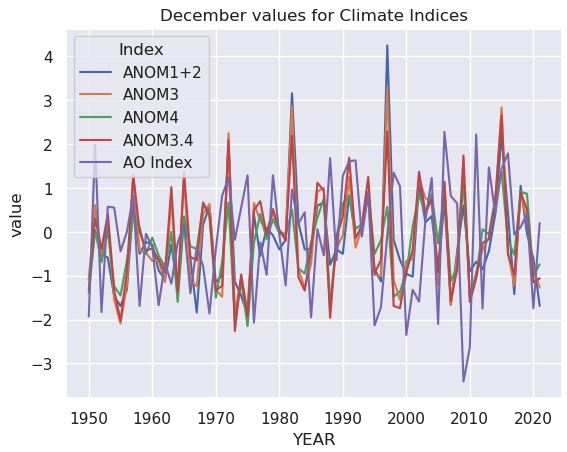
The dark theme with white grid lines is a trademark of Seaborn plots.

Not surprisingly, the various ENSO indices are highly correlated. The Acrtic Oscillation appears it might be anti-correlated with El Niño.

We can display how all these indices relate to each other with the pairplot method. We will go back to our original DataFrame for this, and extract only the anomaly indices for plotting:

columns=['ANOM1+2','ANOM3','ANOM4','ANOM3.4','AO Index']
sns.pairplot(df.query("MONTH == 12")[columns]) ;

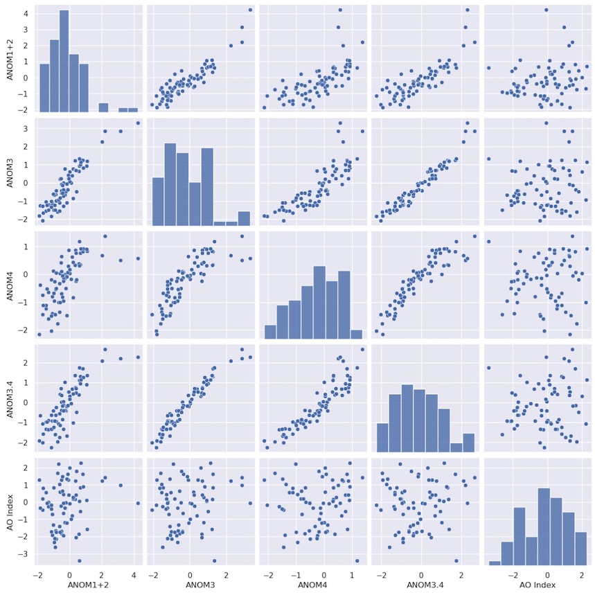
Each index is scattered against every other index. Along the diagonal, a scatter plot would result in a perfect correlation and not reveal any useful new information, so instead a histogram of the probability distribution for each index is plotted automatically.

This is probably not the kind of plot you would use in a presentation or publication, but it is very good for getting a quick look at your data and how the variables might relate. We can see that the El Niño indices are quite well correlated with each other, but the suspected anticorrelation with the AO index is not apparent.

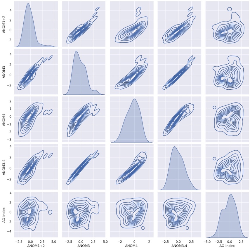
There is an option to plot kernel density instead:

sns.pairplot(df.query("MONTH == 12")[columns], kind="kde") ;

Key Points

• Pandas DataFrames are much like spreadsheets.

• Many of the concepts, and even the names of methods, are the same as for xarray.

• Seaborn provides quick ways to plot the contents of DataFrames.