Where to get Climate Datasets

Overview

Teaching: 15 min
Exercises: 5 min

Questions

• Where do I find Climate Datasets?

Objectives

• Learning to find climate datasets on the web

• How and where to download a dataset from the web

• How to be a good citizen of /homes

Launch a Hopper Desktop session from your ORC Dashboard. We will use it for today’s lesson.

Where can I find Climate Datasets?

Many climate datasets are still available on the COLA servers, and will be migrated to Hopper in the comming months. But how do I find this data? Where would I look to find a dataset that is not on the COLA servers?
As I go forward in my research, how do I find datasets I might want to use?

1. COLA Datasets Catalog
   We are in the process of cataloging all the dataests on the COLA servers. This is a good place to start if you want to know what data are available locally.

2. NOAA/Physical Sciences Lab Many climate datasets are here with lots of information and searching capabilities.

3. IRI/LDEO Climate Data Library This is another great resource for finding Climate Datasets.

4. NCAR Climate Data Guide Great resource for getting expert advice on NCAR’s extensive Climate Data holdings, and which datasets you should use for your specific application.

5. NASA Earth Data NASA has a large distributed archive of Climate Data, mainly from satellites, that is publicly available for download.

Where should I put Climate Datasets?

There are two main ways to access and use climate datasets that are available on the web.

1. You can download a copy of the dataset to your local computer system, and analyze it there.

2. You can access, subset, and (depending on the data server) even analyze the data remotely, having only the result on your local computer system.

Since some climate datasets can be very large, and you may need to use many different ones, option #1 may require a sizeable amount of disk space to store the data. However, once you have a copy of the dataset locally, you own it and you can easily use it over and over.

Option #2 will save space on your computer system, but may also slow down calculations, depending on Internet speed and the load on the remote data servers. It requires reaccessing the data remotely every time you make a change to your calculation.

Thus, there is a decision to be made depending on your situation - one or the other option will be the better choice.

Being a wise computer citizen

If you choose to download data sets to Hopper, recall that your home directory is limited to 50 GB. If you fill up your home disk by downloading too many large datasets there, you may be locked out of the system until you clear space.

Aside from your home directory, there are three other categories of disks which may be a better choice, even for smaller data files:

1. /scratch - for short-term storage of data. There is a nominal 90-day limit for file storage here, and old files are automatically deleted monthly.

2. /tmp - for temporary storage. This disk is mainly used by programs that are running on the cluster that need to temporarily store data on disk as part of their processes. This includes applications like your JupyterLab sessions. If you manually make directories or store files under /tmp, they will remain as long as your session is active, but will disappear as soon as it is not (when your Dashboard session times out, or if you log in via ssh in a terminal session, once your session is closed).

3. /project - for long-term storage of data. Only faculty and research staff can own project directories, which are 1 TB is size. They are associated with a group that includes only users specified by the owner. You should ask your advisor if they have a project disk on Hopper that you can share.

Soon there will be a fourth option. COLA will be moving 1PB of its data holdings to a new disk on Hopper, in late 2022 or early 2023. If you use those data, you will not need to make your own copies on the disk systems listed above.

Downloading Climate Datasets with wget

The most common, and often the easiest, way to download data sets from the web is to use the command wget from a terminal session.

From a terminal window logged in your Hopper desktop, change to the /scratch directory. If you already have your own subdirectory there, go to that. If you do not, make one:

$ cd /scratch
$ mkdir <your_username>
$ cd <your_username>

At one of the data repository websites listed above, let’s find a dataset to download.
In a browser, go to: https://psl.noaa.gov/data/gridded/ and scroll down to the entry: NOAA Extended Reconstructed SST V5. There you will find a web page with a nice description of the dataset.

In the section of the page called “Download/Plot Data”, in the “download file” column you will see two datasets for “Sea Surface Temperature” listed. Click on the download icon for the “Long Term Mean” statistics.

On the new page, you will see a kind of directory listing with several files. Don't click, but right-click on “sst.mon.ltm.1991-2020.nc” and choose “copy link address” to put the URL on your clipboard. Then paste the link into your terminal after typing wget:

$ wget https://downloads.psl.noaa.gov/Datasets/noaa.ersst.v5/sst.mon.ltm.1991-2020.nc

You will get some text on your screen like the following, that reports on the wget process:

[pdirmeye@hop043 pdirmeye]$ wget https://downloads.psl.noaa.gov/Datasets/noaa.ersst.v5/sst.mon.ltm.1991-2020.nc
--2022-08-28 14:09:08--  https://downloads.psl.noaa.gov/Datasets/noaa.ersst.v5/sst.mon.ltm.1991-2020.nc
Resolving downloads.psl.noaa.gov (downloads.psl.noaa.gov)... 140.172.38.86
Connecting to downloads.psl.noaa.gov (downloads.psl.noaa.gov)|140.172.38.86|:443... connected.
HTTP request sent, awaiting response... 200 OK
Length: 1160004 (1.1M) [application/x-netcdf]
Saving to: 'sst.mon.ltm.1991-2020.nc'

sst.mon.ltm.1991-2020.nc 100%[==================================>]   1.11M  4.72MB/s    in 0.2s    

2022-08-28 14:09:09 (4.72 MB/s) - 'sst.mon.ltm.1991-2020.nc' saved [1160004/1160004]

Note that the URL is not http:// or https:// but is ftp://. ftp stands for “file transfer protocol”. It is an old, robust but insecure protocol for moving data that works well from web sites because it has an “anonymous” mode that does not require a user to log in to retrieve files. There is a secure version called sftp that uses ssh and requires passwords. sftp or scp (the secure copy command) are preferred over ftp for moving files between private sources (e.g. your Hopper account and an account you might have at a supercomuting center).

There is a Broswer on Hopper

Note: You have a browser available on your Hopper Desktop. There is a button at the bottom that will launch a Linux build of Firefox. You can use the download capabilities of this browser to download files directly to your Hopper account. This could be a good option if you only have one or a few files to download (that do not require a lot of clicking on links).

However, GUI apps like browsers do not run very smoothly on HPC systems - they are not designed for that. So for larger or more complex downloads where you would benerfit by using wildcards or recursion, It is probably better to use wget from the command line of a terminal window.

Key Points

• Don’t download big datasets to your /homes directory!

Data File Formats

Overview

Teaching: 30 min
Exercises: 0 min

Questions

• What are the common file formats for Climate Datasets?

• What is NetCDF?

• How can we open and access data in NetCDF files?

Objectives

• Become familiar with some of the varieties of data formats used for climate data

• Learn how to peruse and parse a NetCDF file

• Introduction to xarray

Launch a JupyterLab session

Formats of Datasets

There are many data formats in use in the field of climate research, but there are a few that predominate:

1. NetCDF: The Network Common Data Form (originally called the Network Climate Data Format). Typical suffixes: .nc, .nc4. This binary format was developed by the climate community, but has been adopted in many other communities due to its utility and self-describing format (i.e., the data file also includes metadata to describe the contents, its spatial, temporal and any other dimensions, properties and attributes). Beginning with version 4, data compression has become an option. It has become the most common format for climate data files.

2. GRIB: GRIdded Binary format. Typical suffix: grb. GRIB was developed by the World Meteorological Organization (WMO) as an efficient compressed binary format for exchange of weather data. The original format (GRIB1) is only semi-self describing, as it required external look-up tables to decode indices used. GRIB2 is truly self describing. Unlike NetCDF, GRIB allows for tailored compression for each variable in a file.

3. Flat binary files, including those produced as output from FORTRAN programs, and the data files produced by some software packages such as GrADS. No standard suffix. Flat binary files contain no metadata, and usually cannot be understood without additional documntation. The native GrADS file format pairs one or more flat binary data files with a “data descriptor file”, usually ending with the suffix .ctl, that contains all the metadata of a dataset in a human writable and readible form.

4. ASCII files, which include .csv or “comma separated values” files, which are a simple form of storing spreadsheets. ASCII stands for “American Standard Code for Information Interchange”, and is the text or “string” format standard for many programming languages. ASCII is considered easy to read by humans, but is much less efficient at storing data than binary formats. It is advisable only for small files. * In this same category is Unicode, which is an extension of ASCII that uses twich the number of bytes per character, and can accomodate a wide range of languages, symbols, even emojis. This is not very commonly used for storing Earth science data except where storing place names needed extended or alternative alphabets, abjads, syllabaries, etc., are needed.

5. Excel files, a spreadsheet format with a wide range of specialized formatting extensions from Microsoft. Typical suffixes: .xls', .xlsx` (the latter uses extensible markup language XML to encode metadata information).

6. GIS (Geographic Information System) files come in a variety of different formats depending on the application and software used. Often information for a single dataset is split into multiple files, particularly for “shapefiles” containing polygonal data.

7. Orthorectified Imagery Formats such as .tiff files are binary image files used to store geo-located data (also often with metadata in separate files), common for some observational data, especially imagery-derived data from remote sensing or aircraft.

In this course, we will focus on the top part of this list, but know that Python has libraries available to read all these and many more dataset formats.

NetCDF

NetCDF has a software library called NCO (netCDF Operators) that, independent of Python or any other software, can perform a variety of operations on NetCDF datasets. The NCO executables (each function acts like its own Unix command with options and arguments - they even have man and info pages) can be very handy for doing basic operations on data in the bash shell on a Unix system, such as compressing (or “deflating” in NetCDF-speak) a large uncompressed NetCDF dataset you downloaded, in order to conserve disk space.

NCO is available on Hopper as module. To use it, you need to load the module first:

$ module load nco

Perhaps the most useful and often used NCO command is ncdump. Without options, it will dump the entire contents of a NetCDF file to the screen as ASCII numbers and text. The -h option shows only “header” information and not the contents of variables, basically showing you only the metadata.

Strangely, this function is not part of the build on Hopper, but its functionality is contained within the versatile command called ncks (the ks stands for kitchen sink, as it contains everything but the kitchen sink). For ncks, we will use the -m flag, which toggles the printing of the metadata for all variables in the file, behaving like ncdump -h.

Returning to that data file you downloaded to your scratch directory… give it a try:

$ ncks -m sst.mon.ltm.1991-2020.nc

A lot of text is sent to your screen, starting with a list of the dimensions of the dataset in the file, then the variables including a listing of the attributes of each variable.

To see the global attributes of the dataset itself also, use the -M flag:

$ ncks -M sst.mon.ltm.1991-2020.nc

NetCDF metadata

These commands list the metadata in a human-readable format that is fairly easy to interpret.

Find the following information:

1. The names of the dimension variables in the dataset and the size of each
2. The meaning of each dimension variable
3. The data variables (the ones that vary in both space and time dimensions)
4. What is this a dataset of? (peruse the “global attributes”)

Solution

1. lon = 180; lat = 89; time = 12; nbnds = 2
2. lon is longitude (˚E); lat is latitude (˚N); time is months (although that is not terribly obvious from the metadata); nbnds is time boundaries (also a bit mysterious at this point)
3. sst is sea surface temperature [˚C]; valid_yr_count is the “count of non-missing values used in mean”, i.e., number of years of good data used from the 30-year window 1991-2020.
4. A monthly SST climatology averaged over 1991-2020 (the climatology attribute has not been properly updated - it still says 1971-2000) combining several sources of data. It’s called “NOAA Extended Reconstructed SST V5” and there is J. Climate paper describing it.

There are other useful software libraries similar to NCO. In particular, there is the Climate Data Operators (CDO) software package that has much of the same functionality as NCO, but also works with other data formats such as GRIB. It also has a module you can load on Hopper.

Introduction to xarray

To open and use NetCDF datasets in Python, we will use the xarray module. xarray allows for the opening, manipulating and parsing of multi-dimensional datasets that include one or more variables and their associated metadata. In particular, xarray is built with the dask parallel computing library that scales and vectorizes operations on large datasets, making calculations fast and efficient. It provides a very nice balance between ease-of-use and efficiency when analyzing climate datasets.

Open a new Jupyter Notebook and name it “Plot_netcdf.ipynb”.

Before we start, we need to install a bit of software that will help xarray interpret all the information in NetCDF files. In the first code cell, type and run the following:

pip install cftime cfgrib netcdf4 pydap ecmwflibs

Once it has all installed, restart your kernel.

You can comment out that pip line now, as these packages are now installed in your virtual environment and always available.

Then, type the following three import statements:

import numpy as np
import matplotlib.pyplot as plt
import xarray as xr

Note: there is nothing special about the choice of these abbreviations for these three modules - but they happen to be the most commonly used ones by most people. You could use any abbreviation you like, or none at all.

In a new cell, let’s define the path to the dataset we downloaded and open it with xarray:

file = "/scratch/<your_username>/sst.mon.ltm.1981-2010.nc"
ds = xr.open_dataset(file)

Now query the object name ds by typing its name and <return>:

ds

You will get something that looks much like the result of ncks -M, but even more readible.

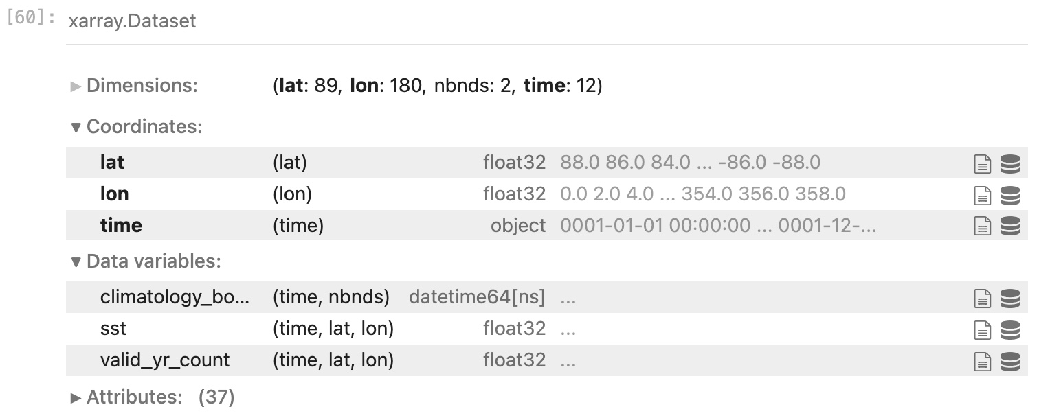
You will also be able to view the contents of any variable, and expand/contract a view of any attributes. For very large or multi-file datasets (xr.open_mfdataset() can open multiple files at once and link them together in a single object), You will also be shown how the data are “chunked” - i.e., organized when loaded into computer memory.

Next, let’s make a plot of the data. To access the variable sst in ds, we can either say:

ds.sst

…or…

ds['sst']

The latter form is more flexible and also makes it clear that ds is not a module with a function called sst – it is less confusing for a human to read. Also, the latter form would allow you to specify the variable name 'sst' as a string variable assigned to that string, which is extremely handy when programming, e.g.:

variable_name = 'sst'
ds[variable_name]

You can see that the dump of ds['sst'] shows more focused information, as well as a sample of the data in the arrays. There are 3 dimensions: time, latitude and longitude (in that sequence - the sequence is important!). To make a 2-D plot, we will choose the first (element 0) time step:

plt.contourf(ds['sst'][0,:,:])

Things to note:

1. contourf is one of the many plotting funtions of matplotlib.pyplot, and especially good for plotting gridded environmental data.
2. The [0,:,:] contruct tells what to do with each dimension of ds['sst'] in order: [time,lat,lon]. * An integer (or variable containing an integer) specifies one index value for that dimension. * : by itself means the entire range. * Sub-ranges are specified with a mix of integers and colons, e.g.: just like with lists, 1: means all but the 0th element, 2:5 would include elements 2-4 (remember it is “up to but not including” the last number). * A second colon could be used to indicate the step, e.g., :10:2 would include elements 0,2,4,6,8 (but not 10).
3. The map is upside down! That is because although there are latitudes and longitudes associated with the last two dimensions of the array, we did not convey that information to the plotting function. Thus, it treats it like a mathematical array with the origin at the lower left. We can also see that the axes are labeled by the indices and not latitudes and longitudes.

We could flip the plot over by changing the indexing of the latitude dimension:

plt.contourf(ds['sst'][0,-1::-1,:])

What does that indexing mean?

• The first -1 means the last element in the latitude dimension. Negative indices are a shortcut to counting from the back instead of the front. The next-to-last element would be -2, etc.
• Nothing between the two colons means proceed to the end, which in this case will be the beginning!
• The second -1 is the step. -1::-1 means count backwards (in this case, start in the south and count north) by ones.

The question mark, and <tab><tab>

In Python, and particularly in Jupyter Notebooks, there are many sources of help as you are writing code. Two that are especially useful:

• If you place a question mark immediately after an object (Python is an “object-oriented” programming language, and everything in Python is an “object”), in most cases you will get a brief, helpful description of it. The degree of detail will vary, but it can help you to keep straight and understand what is what.
• If you are typing the name of a function and halfway through you don’t quite remember the spelling or syntax, you can hit the tab twice and a list of auto-complete options will come up to help you. You can click on the one you want to finish typing it.

Key Points

• NetCDF is now the most common climate data format.

• xarray wants to be your best friend - let it!

OPeNDAP and GRIB

Overview

Teaching: 20 min
Exercises: 0 min

Questions

• How can we use OpenDap to access dataset directly across the web?

• How do we open GRIB files?

Objectives

• Learn how to use xarray to read remote datasets

• Learn how to use xarray to read GRIB files

OPeNDAP

OPeNDAP (Open-source Project for a Network Data Access Protocol) is s a data server architecture that allows access to remote datasets within many different software packages including Python.
Opening a remote file via OPeNDAP is as easy as opening a file on local disk, except a URL to the dataset is supplied instead of a path on local disk. Regardless of the native data file format, OPeNDAP presents it to the client software in a NetCDF-style format.

When a file is opened via OPeNDAP, only the metadata is initially passed to the client. Just the specific slices of variables used in a calculation are sent over the Internet, not the entire dataset. Thus, it can be much more efficient than downloading a large dataset and only using a small part of it. However, performance of code using OPeNDAP depends on the speed of the Internet connection to the data server.

OPeNDAP in xarray

To open and use remote datasets in Python served via OPeNDAP, we use the xarray function open_dataset() in exactly the same way as before. This time, let’s look at a different dataset from the NOAA PSL repository. Let’s look at the Palmer Drought Severity Index page and select the OPeNDAP file name for the self-calibrated version.

In a new code cell, type the following (you can copy and paste the dataset path from the web page):

url = "https://psl.noaa.gov/thredds/dodsC/Datasets/dai_pdsi/pdsi.mon.mean.selfcalibrated.nc"
dd = xr.open_dataset(url)

This may have taken a few seconds, whereas opening the local file was nearly instantaneous. There was some communication over the Internet to establish a link between your Python process running in a Jupyter Notebook on Hopper and the remote data server (which sits in Boulder, Colorado).

As before, query the new object dd by typing its name and <return>:

dd

In the same format as before you will see the metadata pertinent to this dataset. There is only one data variable, the horizontal resolution is a bit lower (the spatial dimensions of the arrays are smaller) but the time dimension is much larger.

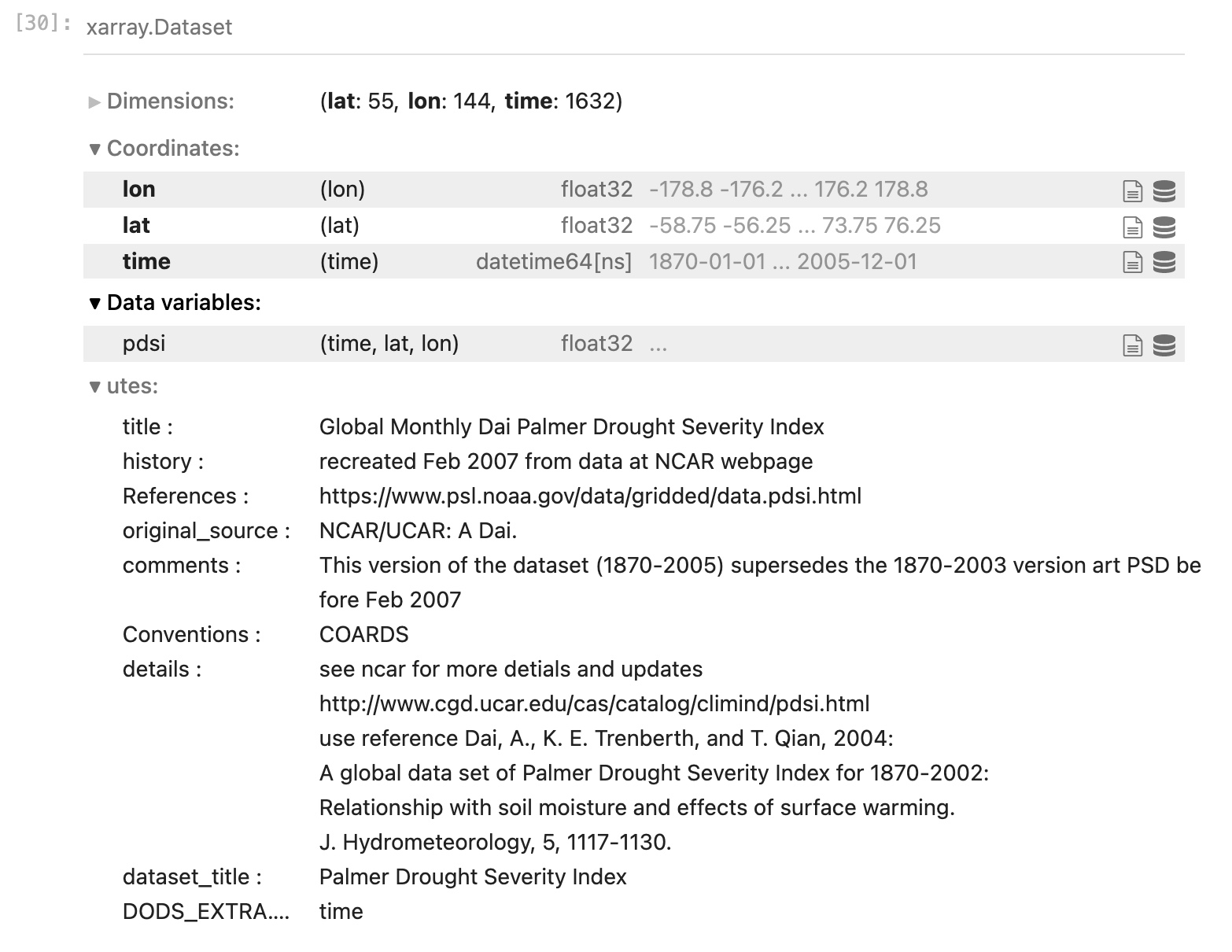
The dimensions of this data are again in the order: [time, lat, lon] (always check before you move forward!), so we may make a quick plot of this data. This time, let’s plot the last time step:

plt.contourf(dd["pdsi"][-1,:,:]) ; plt.colorbar()

Things to note: 1. There was more hesitation - although the spatial grid is smaller than the SST data we downloaded to disk, we had to retrieve the data over the Internet. If we were only interested in the last month, or last year, of this 164-year dataset, this would be more efficient than downloading the whole file first. However, if we wanted to do a number of different calculations using the whole time series, it might be better in the long run to download it. 2. It’s not upside down! If you noticed when you queried the metadata, the latitudes start at -58.75 and count up to 76.25. So we also see it is not a full global grid, but it excludes Antarctica and areas north of the Arctic Circle. 3. We added a colorbar using a different pyplot function. 4. Also note that we put two separate Python commands on the same line separated by a semicolon. This is valid syntax in Python - you do not have to have one command per line.

Opening a GRIB file in xarray

GRIB format is used by operational weather forecast centers around the world for forecast model output. Let’s go back to our terminal window and copy the following file to your scratch directory:

$ cd /scratch/<your_username>
$ cp /home/pdirmeye/classes/clim680_2022/ei.oper.an.pl.regn128cm.2014020800 test.grb

Back in our Jupyter notebook, let’s open a new code cell and proceed to open this GRIB file containing data from the ERA-Interim reanalysis from ECMWF:

gribfile = "/scratch/<your_username>/test.grb"
dg = xr.open_dataset(gribfile,engine='cfgrib')

We had to specify an “engine” that knows how to read a GRIB file. If you look in your scratch directory, you will find a new file has been created. Because GRIB files are extremely compressed, down to the bit level, an index file (ending in .idx) is generated from the metadata that holds a mapping of the exact places on disk where each grid starts, and specific information on how to uncompress each grid. This speeds up the navigation and processing of the dataset.

Examine the file’s metadata:

dg

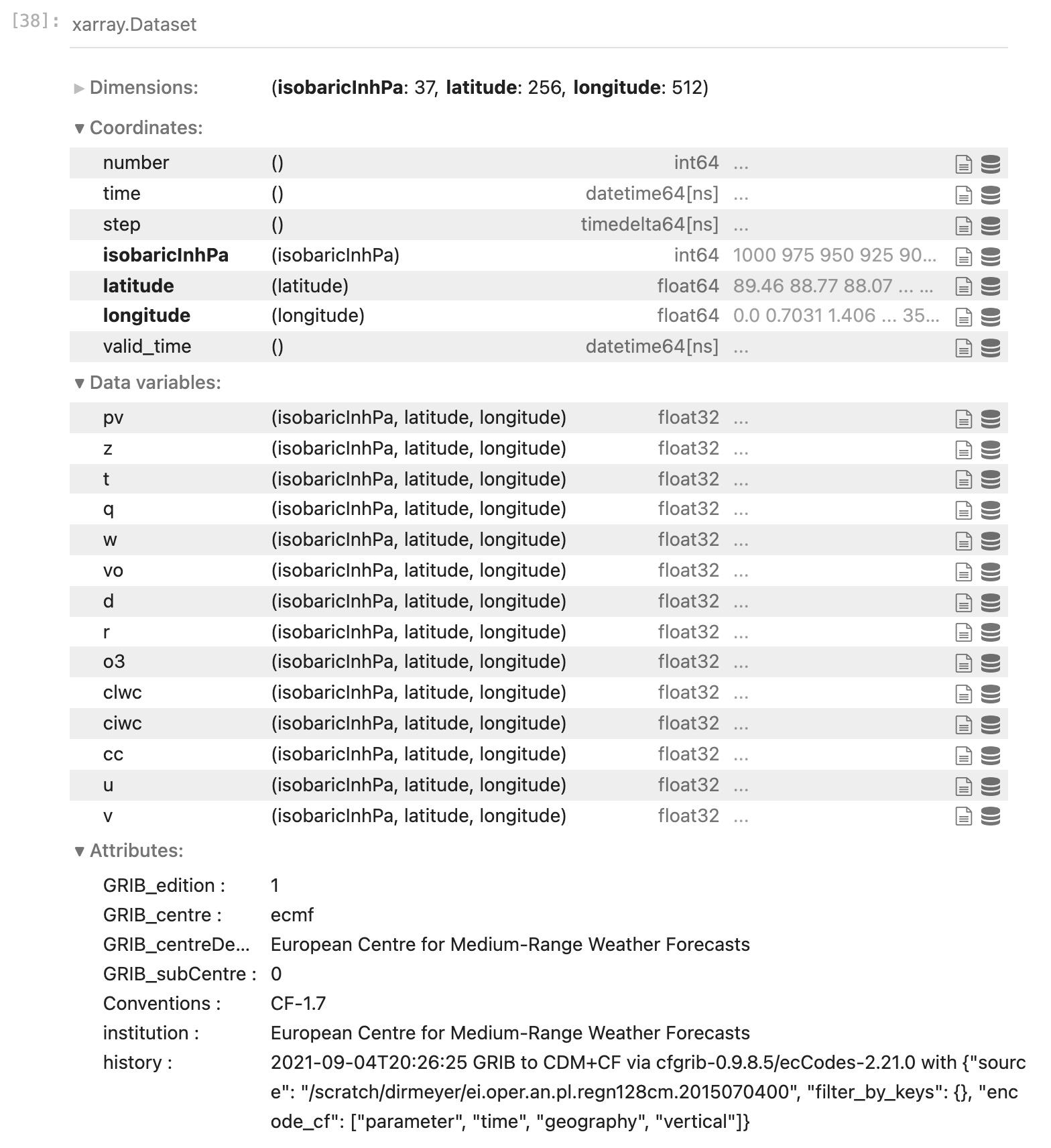
Note that here we again have 3 dimensions, but time is not one of them. These are global grids at a single date/time, but across 37 pressure levels (the coordinate isobaricInhPa)

Expand the attributes of any data variable and have a look.

Finally, make a plot of one of the variables at a particlar pressure level (something you might be familiar with like t temperature or u zonal wind). Do you remember the syntax? Can you add a colorbar?

Key Points

• OPeNDAP allows remote access to datasets across the Internet without downloading files.

• xarray renders differences between local and remote data, and between different data file formats nearly imperceptable.